Creating TNT elements using Basix’s custom element interface
This demo (demo_tnt-elements.py) illustrates how to:
Define custom finite elements using Basix
We begin this demo by importing everything we require.
import matplotlib.pylab as plt
import numpy as np

import basix
import basix.ufl_wrapper
from dolfinx import fem, mesh
from ufl import (SpatialCoordinate, TestFunction, TrialFunction, cos, div, dx,
                 grad, inner, sin)

from mpi4py import MPI
Defining a degree 1 TNT element
Basix supports a range of finite elements, but there are many other possible elements a user may want to use. This demo shows how the Basix custom element interface can be used to define elements. More detailed information about the inputs needed to create a custom element can be found in the Basix documentation.
As an example, we will define tiniest tensor (TNT) elements on a quadrilateral, as defined in Commuting diagrams for the TNT elements on cubes (Cockburn, Qiu, 2014).
The polynomial set
We begin by defining a basis of the polynomial space that this element spans. This is defined in terms of the orthogonal Legendre polynomials on the cell. For a degree 1 TNT element, the polynomial set contains the polynomials \(1\), \(y\), \(y^2\), \(x\), \(xy\), \(xy^2\), \(x^2\), and \(x^2y\). These are the first 8 polynomials in the degree 2 set of polynomials on a quadrilateral, so we create an 8 by 9 (number of dofs by number of polynomials in the degree 2 set) matrix with an 8 by 8 identity in the first 8 columns. The order in which polynomials appear in the polynomial sets for each cell can be found in the Basix documentation.
wcoeffs = np.eye(8, 9)
The interpolation operators
Next, we provide the information that defines the DOFs associated with each sub-entity of the cell. We first associate a point evaluation with each vertex of the cell.
geometry = basix.geometry(basix.CellType.quadrilateral)
topology = basix.topology(basix.CellType.quadrilateral)
x = [[], [], [], []]  # type: ignore [var-annotated]
M = [[], [], [], []]  # type: ignore [var-annotated]

for v in topology[0]:
    x[0].append(np.array(geometry[v]))
    M[0].append(np.array([[[[1.]]]]))
For each edge of the cell, we define points and a matrix that represent the integral of the function along that edge. We do this by mapping quadrature points to the edge and putting quadrature points in the matrix.
pts, wts = basix.make_quadrature(basix.CellType.interval, 1)
for e in topology[1]:
    v0 = geometry[e[0]]
    v1 = geometry[e[1]]
    edge_pts = np.array([v0 + p * (v1 - v0) for p in pts])
    x[1].append(edge_pts)

    mat = np.zeros((1, 1, pts.shape[0], 1))
    mat[0, 0, :, 0] = wts
    M[1].append(mat)
There are no DOFs associated with the interior of the cell for the lowest order TNT element, so we associate an empty list of points and an empty matrix with the interior.
x[2].append(np.zeros([0, 2]))
M[2].append(np.zeros([0, 1, 0, 1]))
Creating the Basix element
We now create the element. Using the Basix UFL interface, we can wrap this element so that it can be used with FFCx/DOLFINx.
e = basix.create_custom_element(basix.CellType.quadrilateral, [], wcoeffs, x, M,
                                0, basix.MapType.identity, False, 1, 2)
tnt_degree1 = basix.ufl_wrapper.BasixElement(e)
Creating higher degree TNT elements
The following function follows the same method as above to define arbitrary degree TNT elements.
def create_tnt_quad(degree):
    assert degree > 1
    # Polyset
    ndofs = (degree + 1) ** 2 + 4
    npoly = (degree + 2) ** 2

    wcoeffs = np.zeros((ndofs, npoly))

    dof_n = 0
    for i in range(degree + 1):
        for j in range(degree + 1):
            wcoeffs[dof_n, i * (degree + 2) + j] = 1
            dof_n += 1

    for i, j in [(degree + 1, 1), (degree + 1, 0), (1, degree + 1), (0, degree + 1)]:
        wcoeffs[dof_n, i * (degree + 2) + j] = 1
        dof_n += 1

    # Interpolation
    geometry = basix.geometry(basix.CellType.quadrilateral)
    topology = basix.topology(basix.CellType.quadrilateral)
    x = [[], [], [], []]
    M = [[], [], [], []]

    # Vertices
    for v in topology[0]:
        x[0].append(np.array(geometry[v]))
        M[0].append(np.array([[[[1.]]]]))

    # Edges
    pts, wts = basix.make_quadrature(basix.CellType.interval, 2 * degree - 1)
    poly = basix.tabulate_polynomials(basix.PolynomialType.legendre, basix.CellType.interval, degree - 1, pts)
    edge_ndofs = poly.shape[1]
    for e in topology[1]:
        v0 = geometry[e[0]]
        v1 = geometry[e[1]]
        edge_pts = np.array([v0 + p * (v1 - v0) for p in pts])
        x[1].append(edge_pts)

        mat = np.zeros((edge_ndofs, 1, len(pts), 1))
        for i in range(edge_ndofs):
            mat[i, 0, :, 0] = wts[:] * poly[i, :]
        M[1].append(mat)

    # Interior
    if degree == 1:
        x[2].append(np.zeros([0, 2]))
        M[2].append(np.zeros([0, 1, 0, 1]))
    else:
        pts, wts = basix.make_quadrature(basix.CellType.quadrilateral, 2 * degree - 2)
        poly = basix.tabulate_polynomials(basix.PolynomialType.legendre, basix.CellType.quadrilateral, degree - 2, pts)
        face_ndofs = poly.shape[0]
        x[2].append(pts)
        mat = np.zeros((face_ndofs, 1, len(pts), 1))
        for i in range(face_ndofs):
            mat[i, 0, :, 0] = wts[:] * poly[i, :]
        M[2].append(mat)

    e = basix.create_custom_element(
        basix.CellType.quadrilateral, [], wcoeffs, x, M, 0, basix.MapType.identity, False, degree, degree + 1)
    return basix.ufl_wrapper.BasixElement(e)
Comparing TNT elements and Q elements
We now use the code above to compare TNT elements and Q elements on quadrilaterals.
The following function takes a DOLFINx function space as input, and solves a Poisson problem and returns the \(L_2\) error of the solution.
def poisson_error(V):
    msh = V.mesh
    u, v = TrialFunction(V), TestFunction(V)

    x = SpatialCoordinate(msh)
    u_exact = sin(10 * x[1]) * cos(15 * x[0])
    f = - div(grad(u_exact))

    a = inner(grad(u), grad(v)) * dx
    L = inner(f, v) * dx

    # Create Dirichlet boundary condition
    u_bc = fem.Function(V)
    u_bc.interpolate(lambda x: np.sin(10 * x[1]) * np.cos(15 * x[0]))

    msh.topology.create_connectivity(msh.topology.dim - 1, msh.topology.dim)
    bndry_facets = mesh.exterior_facet_indices(msh.topology)
    bdofs = fem.locate_dofs_topological(V, msh.topology.dim - 1, bndry_facets)
    bc = fem.dirichletbc(u_bc, bdofs)

    # Solve using LU linear solver
    problem = fem.petsc.LinearProblem(a, L, bcs=[bc], petsc_options={"ksp_type": "preonly", "pc_type": "lu"})
    uh = problem.solve()

    M = (u_exact - uh)**2 * dx
    M = fem.form(M)
    error = msh.comm.allreduce(fem.assemble_scalar(M), op=MPI.SUM)
    return error**0.5
We create a mesh, then solve the Poisson problem using our TNT elements of degree 1 to 8. We then do the same with Q elements of degree 1 to 9. For the TNT elements, we store a number 1 larger than the degree as this is the highest degree polynomial in the space.
msh = mesh.create_unit_square(MPI.COMM_WORLD, 15, 15, mesh.CellType.quadrilateral)

tnt_ndofs = []
tnt_degrees = []
tnt_errors = []

V = fem.FunctionSpace(msh, tnt_degree1)
tnt_degrees.append(2)
tnt_ndofs.append(V.dofmap.index_map.size_global)
tnt_errors.append(poisson_error(V))
print(f"TNT degree 2 error: {tnt_errors[-1]}")

for degree in range(2, 9):
    V = fem.FunctionSpace(msh, create_tnt_quad(degree))

    tnt_degrees.append(degree + 1)
    tnt_ndofs.append(V.dofmap.index_map.size_global)
    tnt_errors.append(poisson_error(V))
    print(f"TNT degree {degree} error: {tnt_errors[-1]}")

q_ndofs = []
q_degrees = []
q_errors = []
for degree in range(1, 10):
    V = fem.FunctionSpace(msh, ("Q", degree))
    q_degrees.append(degree)
    q_ndofs.append(V.dofmap.index_map.size_global)
    q_errors.append(poisson_error(V))
    print(f"Q degree {degree} error: {q_errors[-1]}")
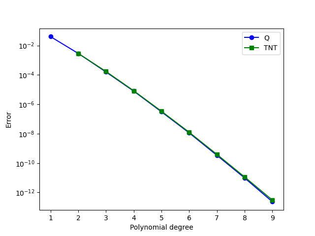
We now plot the data that we have obtained. First we plot the error against the polynomial degree for the two elements. The two elements appear to perform equally well.
if MPI.COMM_WORLD.rank == 0:  # Only plot on one rank
    plt.plot(q_degrees, q_errors, "bo-")
    plt.plot(tnt_degrees, tnt_errors, "gs-")

    plt.yscale("log")
    plt.xlabel("Polynomial degree")
    plt.ylabel("Error")
    plt.legend(["Q", "TNT"])

    plt.savefig("demo_tnt-elements_degrees_vs_error.png")
    plt.clf()
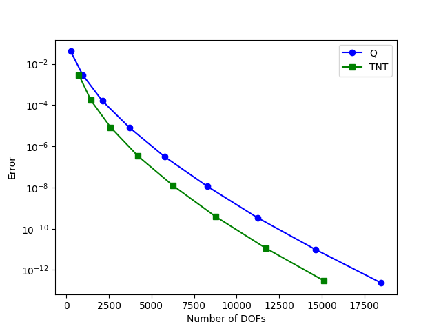
A key advantage of TNT elements is that for a given degree, they span a smaller polynomial space than Q elements. This can be observed in the following diagram, where we plot the error against the number of DOFs.
if MPI.COMM_WORLD.rank == 0:  # Only plot on one rank
    plt.plot(q_ndofs, q_errors, "bo-")
    plt.plot(tnt_ndofs, tnt_errors, "gs-")

    plt.yscale("log")
    plt.xlabel("Number of DOFs")
    plt.ylabel("Error")
    plt.legend(["Q", "TNT"])

    plt.savefig("demo_tnt-elements_ndofs_vs_error.png")
    plt.clf()