Defining conforming Crouzeix–Raviart elements

In this demo, we show how Basix’s custom element functionality can be used to create a conforming Crouzeix–Raviart element.

First, we import Basix and Numpy.

import basix
import numpy as np
from basix import CellType, MapType, PolynomialType, LatticeType

from mpl_toolkits import mplot3d  # noqa: F401
import matplotlib.pyplot as plt

Conforming CR element on a triangle

We begin by implementing this element on a triangle. The following function implements this element for an arbitrary degree. Details of the definition of this element can be found at https://defelement.com/elements/conforming-crouzeix-raviart.html.

As the input to this function, we use the degree of the element as shown on DefElement. For most degrees, the highest degree polynomial in this elements polynomial space is actually one degree higher, so we pass degree + 1 into create_custom_element.

def create_ccr_triangle(degree):

    if degree == 1:
        wcoeffs = np.eye(3)

        x = [[], [], [], []]
        x[0].append(np.array([[0.0, 0.0]]))
        x[0].append(np.array([[1.0, 0.0]]))
        x[0].append(np.array([[0.0, 1.0]]))

        for _ in range(3):
            x[1].append(np.zeros((0, 2)))
        x[2].append(np.zeros((0, 2)))

        M = [[], [], [], []]
        for _ in range(3):
            M[0].append(np.array([[[1.]]]))

        for _ in range(3):
            M[1].append(np.zeros((0, 1, 0)))
        M[2].append(np.zeros((0, 1, 0)))

        return basix.create_custom_element(
            CellType.triangle, [], wcoeffs, x, M, MapType.identity, False, 1, 1)

    npoly = (degree + 2) * (degree + 3) // 2
    ndofs = degree * (degree + 5) // 2
    wcoeffs = np.zeros((ndofs, npoly))

    dof_n = 0
    for i in range((degree + 1) * (degree + 2) // 2):
        wcoeffs[dof_n, dof_n] = 1
        dof_n += 1

    pts, wts = basix.make_quadrature(CellType.triangle, 2 * (degree + 1))
    poly = basix.tabulate_polynomials(PolynomialType.legendre, CellType.triangle, degree + 1, pts)
    for i in range(1, degree):
        x = pts[:, 0]
        y = pts[:, 1]
        f = x ** i * y ** (degree - i) * (x + y)

        for j in range(npoly):
            wcoeffs[dof_n, j] = sum(f * poly[:, j] * wts)
        dof_n += 1

    geometry = basix.geometry(CellType.triangle)
    topology = basix.topology(CellType.triangle)
    x = [[], [], [], []]
    M = [[], [], [], []]
    for v in topology[0]:
        x[0].append(np.array(geometry[v]))
        M[0].append(np.array([[[1.]]]))
    pts = basix.create_lattice(CellType.interval, degree, LatticeType.equispaced, False)
    mat = np.zeros((len(pts), 1, len(pts)))
    mat[:, 0, :] = np.eye(len(pts))
    for e in topology[1]:
        edge_pts = []
        v0 = geometry[e[0]]
        v1 = geometry[e[1]]
        for p in pts:
            edge_pts.append(v0 + p * (v1 - v0))
        x[1].append(np.array(edge_pts))
        M[1].append(mat)
    pts = basix.create_lattice(CellType.triangle, degree + 1, LatticeType.equispaced, False)
    x[2].append(pts)
    mat = np.zeros((len(pts), 1, len(pts)))
    mat[:, 0, :] = np.eye(len(pts))
    M[2].append(mat)

    return basix.create_custom_element(
        CellType.triangle, [], wcoeffs, x, M, MapType.identity, False, degree, degree + 1)

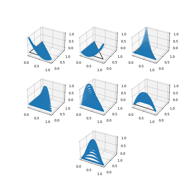
We can then create a degree 2 conforming CR element.

e = create_ccr_triangle(2)

We now visualise the basis functions of the element we have created.

pts = basix.create_lattice(CellType.triangle, 30, LatticeType.equispaced, True)

x = pts[:, 0]
y = pts[:, 1]
z = e.tabulate(0, pts)[0]

fig = plt.figure(figsize=(8, 8))

for n in range(7):
    if n == 6:
        ax = plt.subplot(3, 3, n + 2, projection='3d')
    else:
        ax = plt.subplot(3, 3, n + 1, projection='3d')
    ax.plot([0, 1, 0, 0], [0, 0, 1, 0], [0, 0, 0, 0], "k-")
    ax.scatter(x, y, z[:, n, 0])

plt.savefig("ccr_triangle_2.png")

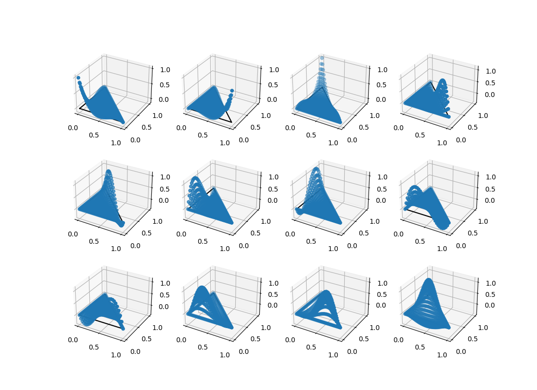
We also visualise the basis functions of a degree 3 conforming CR element.

e = create_ccr_triangle(3)

pts = basix.create_lattice(CellType.triangle, 30, LatticeType.equispaced, True)

x = pts[:, 0]
y = pts[:, 1]
z = e.tabulate(0, pts)[0]

fig = plt.figure(figsize=(11, 8))

for n in range(12):
    ax = plt.subplot(3, 4, n + 1, projection='3d')
    ax.plot([0, 1, 0, 0], [0, 0, 1, 0], [0, 0, 0, 0], "k-")
    ax.scatter(x, y, z[:, n, 0])

plt.savefig("ccr_triangle_3.png")